Q1. Define forecasting. What are the main goals and applications of forecasting in business and economics?
Forecasting:
Forecasting is the process of predicting future events or trends based on historical data, analysis, and models.
Main Goals of Forecasting:
1️⃣ Future Planning:
To estimate future demand, sales, or production needs.
2️⃣ Risk Reduction:
Helps to reduce uncertainty by providing data-based insights.
3️⃣ Better Decision-Making:
Assists managers and policymakers in making strategic choices.
4️⃣ Resource Allocation:
Helps in proper budgeting and resource management.
5️⃣ Performance Improvement:
Businesses can track and improve future performance by learning from trends.
Applications in Business and Economics:
Sales forecasting to plan production and inventory
Financial forecasting for budgeting and investment decisions
Economic forecasting for GDP, inflation, and employment trends
Supply chain management for demand planning
Marketing strategy and product launches based on trend predictions
Q2. Differentiate between qualitative and quantitative forecasting methods. Give two examples of each.
Qualitative Forecasting Methods
What is it?
These methods are based on human judgment, opinions, and intuition, not on historical data. They are used when past data is not available or when forecasting new products, trends, or situations. When to use?
When historical data is missing or unreliable
When launching a new product or entering a new market
When expert opinion is more useful than past patterns Examples:
Delphi Method – A panel of experts is asked to give their opinions anonymously. Their responses are collected, summarized, and shared in rounds until a consensus forecast is reached.
Market Research – Surveys or interviews with customers to predict demand or trends based on what people say they will do or prefer.
Quantitative Forecasting Methods
What is it?
These methods use mathematical models and historical data to make forecasts. They rely on data patterns, trends, seasonality, and statistics. When to use?
When you have enough reliable historical data
When patterns like trends or seasonality exist
When you want data-driven, objective results Examples:
Moving Average – Takes the average of previous values (like sales over last 3 months) to predict the next value.
Exponential Smoothing – Assigns more weight to recent data and less to older data to forecast future values more accurately.
Summary:
Basis
Qualitative Forecasting
Quantitative Forecasting
Definition
Based on expert opinions, intuition, or judgment.
Based on mathematical models and historical data.
Data Required
Does not require numerical data.
Requires past numerical data for calculations.
Usefulness
Useful when data is not available or future is uncertain.
Useful when past trends can be analyzed.
Accuracy
Less accurate; subjective.
More accurate; objective and data-driven.
Examples
1. Delphi Method
1. Time Series Analysis 2. Regression Analysis
Conclusion:
Qualitative methods rely on opinions and experience, while quantitative methods use mathematical models and data for forecasting.
Q3. Explain the variate component method in time series analysis. What are its key components?
What is Variate Component Method?
It is a method in time series analysis where we break the time series data into parts (called components) so we can understand and analyze each part separately.
The Variate Component Method is a technique used in time series analysis to break down (decompose) a time series into its individual components to better understand patterns and make predictions.
Key Components of Time Series:
1️⃣ Trend (T):
It shows the long-term movement or direction of the data over time.
Slow and steady increase or decrease in data over a long time.
Example: Gradual increase in sales over years.
2️⃣ Seasonal Component (S):
It refers to regular patterns that repeat at fixed periods (like months or quarters).
Patterns that repeat regularly in a fixed time (like every year or month)
Example: Increase in ice-cream sales during summer.
3️⃣ Cyclical Component (C):
It refers to long-term up and down movements not of fixed period, usually related to the business cycle.
Ups and downs in data over a long time but not in a fixed pattern.
Example: Economic booms or recessions.
4️⃣ Irregular/Random Component (I):
It includes Unexpected or random changes in the data
Example: Sudden drop in sales due to natural disaster.
Models Used:
**Additive Model:**This model expresses a time series as the sum of its trend, seasonal, cyclical, and irregular components.
Y=T+S+C+I
Multiplicative Model:: This model expresses a time series as the product of its trend, seasonal, cyclical, and irregular components, often used when variations change proportionally with the series magnitude.
Y=T×S×C×I
(Used when variations increase or decrease with time)
Conclusion:
The Variate Component Method helps to analyze and forecast time series by studying each component separately, improving understanding of the data behavior.
Q4. When would you choose an additive model over a multiplicative model in time series decomposition? Explain with examples.
Use Additive Model when:
The change (up or down) is always the same amount, no matter how big or small the overall values are.
Use when seasonal and irregular variations are constant over time. Example:
Every December, a shop sells 100 extra books for Christmas — always +100, not more or less depending on the year.
So, use Additive model: Sales = Trend + Seasonal + Irregular + Cyclical
Use Multiplicative Model when:
The change is a percentage of the total — it grows or shrinks as the trend grows.
Use when seasonal or irregular variations increase or decrease with the trend. Example:
A shop sees a 20% increase in summer sales every year.
If normal sales are 1000, summer sales = 1200.
If normal sales grow to 2000, summer sales = 2400.
So, use Multiplicative model: Sales = Trend × Seasonal × Irregular x Cyclical
In short:
Additive = fixed amount change
Multiplicative = percentage change
Q5. What is a stationary time series? Distinguish between strict stationarity and weak stationarity.
Stationary Time Series (Simple Explanation):
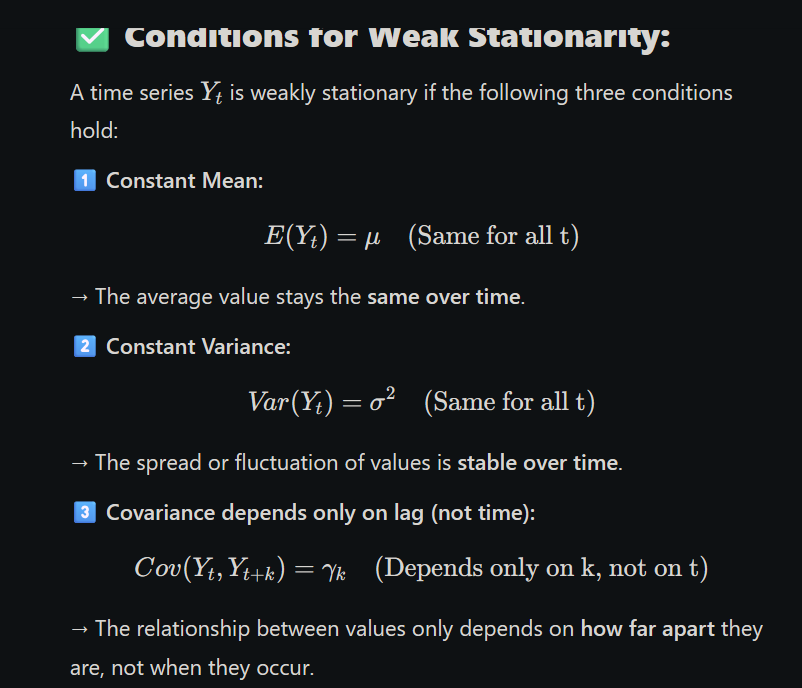
A stationary time series is one where the data’s key properties do not change over time — specifically:
Mean (average) stays constant
Variance (spread of data) stays constant
Covariance (relationship between values at different times) depends only on the time gap, not the actual time
Types of Stationarity:
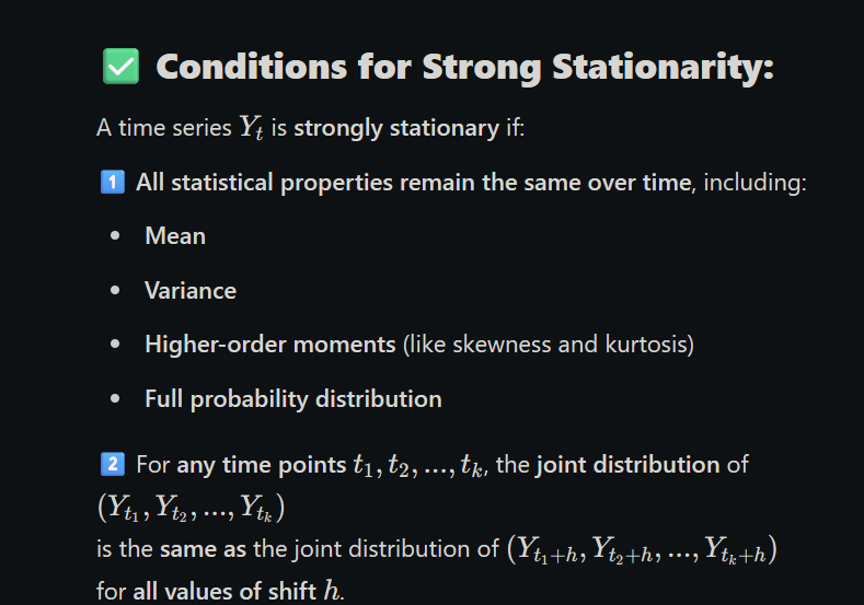
1. Strict Stationarity:
Strict Stationarity) means that the entire distribution of a time series remains the same over time — not just the mean or variance, but all moments and joint distributions.
The entire distribution (not just mean/variance) stays the same over time.
All statistical properties are unchanged if we shift time. Example: If the data pattern looks the same whether you look at day 1–10 or day 100–110, it is strictly stationary.
2. Weak Stationarity (also called Covariance Stationarity):
Weak Stationarity (also called Second-order Stationarity) means that a time series has constant statistical properties over time — specifically mean, variance, and covariance.
Only the mean, variance, and covariance are constant over time.
This is more commonly used in practice. Example: A series with constant average sales and similar ups/downs over time is weakly stationary.
Key Differences:
Feature
Strict Stationarity
Weak Stationarity
Based on
Full distribution
Mean, variance, and covariance only
Strict conditions
Yes
Relaxed conditions
Usage in practice
Rarely checked (hard to test)
Often used in models like ARIMA
Q6. Define autocorrelation function (ACF). How does it help in identifying the structure of a time series?
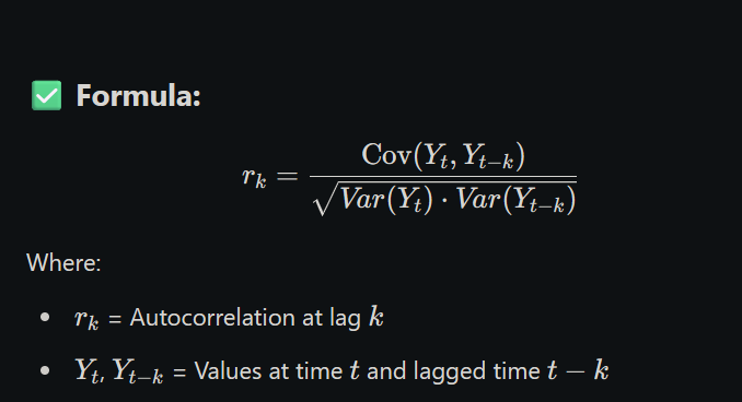
✅ Definition:
The Autocorrelation Function (ACF) measures the correlation between a time series and its past values (lags).
It tells us how much the present value of the series is related to its past values.
In simple words:
ACF shows how current data points are similar or related to previous ones over different time gaps (lags).
✅ Formula:
How ACF Helps in Time Series Analysis
🔍 1. Identifying Time Series Patterns:
Helps detect trend, seasonality, or randomness.
High autocorrelation at certain lags indicates repeating patterns.
🧱 2. Model Selection:
ACF plot (called Correlogram) helps in choosing models like:
AR (Autoregressive) → if ACF decreases gradually.
MA (Moving Average) → if ACF cuts off after a few lags.
ARMA/ARIMA → combined behavior.
📉 3. Checking Stationarity:
If ACF drops to zero quickly, the series is likely stationary.
If ACF stays high → non-stationary (needs differencing).
✅ Conclusion:
The Autocorrelation Function is a key tool in time series analysis. It helps to understand structure, choose models, and test if data is stationary or not.
Q7. What is a correlogram? How is it useful in time series analysis?
Definition:
A correlogram is a graphical representation of the autocorrelation function (ACF) of a time series. It shows how correlated the current value is with its past values (lags), plotted against the number of lags.
How it is Useful in Time Series Analysis:
Detects Serial Correlation:
Helps identify if data points are related to previous values.
Checks Stationarity:
If autocorrelations drop quickly (cut off), the series may be stationary. If they decay slowly, the series is likely non-stationary.
Identifies Seasonality:
Regular repeating spikes at specific lags suggest seasonal patterns.
Model Selection:
Helps decide the order of AR (AutoRegressive) or MA (Moving Average) components for ARIMA models.
Visual Diagnostic Tool:
Makes it easier to understand autocorrelation behavior instead of reading values from a table.
Example:
A correlogram showing strong spikes at lag 12, 24, etc., may indicate yearly seasonality in monthly sales data.
Note
simple exponential smoothing:
a method to forecast when data has no trend or seasonality. it gives more weight to recent values and less to older ones. used when data stays mostly stable over time.
holt’s double exponential smoothing:
an improved version that works when data has a trend. it smooths both the level and the trend to give better forecasts. used when values are steadily increasing or decreasing.
Here is a simple, exam-ready answer for 5 marks on Brown’s Discounted Regression:
Brown’s Discounted Regression
✅ Definition:
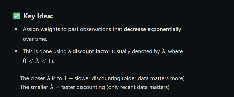
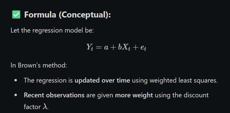
Brown’s Discounted Regression is a forecasting method that gives more weight to recent data and less weight to older data using a discounting factor.
It is often used when recent trends are more important than older patterns, especially in changing environments.
✅ Key Idea:
.
✅ Formula (Conceptual):
✅ Uses:
Short-term forecasting in dynamic environments.
Helpful when data has trending behavior or recent changes are important.
✅ Advantages:
Quick to update forecasts with new data.
Gives more importance to recent trends.
Suitable for real-time decision-making.
❌ Disadvantages:
Not suitable for data with seasonality.
Choosing the right discount factor is critical.
Less effective if past data is equally important.
✅ Conclusion:
Brown’s Discounted Regression is a practical forecasting method that adjusts predictions by discounting older data, making it ideal for fast-changing time series.
Q8. Compare simple exponential smoothing and Holt’s double exponential smoothing. When is each method appropriate?
Comparison: Simple Exponential Smoothing vs. Holt’s Double Exponential Smoothing
Feature
Simple Exponential Smoothing (SES)
Holt’s Double Exponential Smoothing
Trend Handling
Does not handle trend
Handles linear trend
Components Used
Only level
Level + Trend
Complexity
Simple to apply
More complex (uses two smoothing constants)
Forecast Equation
Based on weighted average of past values
Adds a trend term to the forecast
When to Use
For stationary data (no trend/seasonality)
For data with a trend (but no seasonality)
When is Each Method Appropriate?
Simple Exponential Smoothing (SES):
Use when the data has no clear trend or seasonality — e.g., stable monthly demand for a basic item.
Holt’s Double Exponential Smoothing:
Use when the data shows a consistent upward or downward trend — e.g., steadily increasing product sales over time.
Example:
SES: Daily electricity usage in a factory with stable demand.
Holt’s: Monthly revenue of a growing company.
Q9. Discuss any two exponential smoothing methods to forecast the future data.
1. simple exponential smoothing:
this method is used when the data has no trend or seasonality. it gives more weight to recent values and less to older ones using a smoothing factor called alpha (α), which lies between 0 and 1.
the formula is:
forecast = α × current actual value + (1 − α) × previous forecast
if α is close to 1, more weight is given to the recent data.
this method is easy to apply and best suited for short-term forecasts where data is steady without much change. example:
forecasting daily demand for bread in a shop where sales are usually around 100 units with small variations. advantages:
easy to compute
works well for stable time series
requires less data limitations:
does not work if there is trend or seasonality in data
2. holt’s double exponential smoothing:
this is an extension of simple exponential smoothing and is used when the data has a trend (either upward or downward). it uses two equations — one for the current level and one for the trend.
it uses two smoothing constants:
alpha (α) for the level
beta (β) for the trend
the forecast is adjusted by both the current level and the trend value. it is more accurate than simple exponential smoothing when there is a clear trend. example:
forecasting monthly sales of a product that increases by 20 units every month. advantages:
captures both level and trend
better accuracy for trending data
suitable for short to medium-term forecasting limitations:
Q1. Given a time series Y = [5, 6, 4, 7, 6, 5, 4, 6, 5, 6], compute the mean and variance. Verify if the mean and variance are constant.
Given Data
Time Series Y = [5, 6, 4, 7, 6, 5, 4, 6, 5, 6] n = 10 observations
Step 1: Calculate Overall Mean and Variance
Mean Calculation Table
t
Yₜ
1
5
2
6
3
4
4
7
5
6
6
5
7
4
8
6
9
5
10
6
Total
54
Overall Mean (Ȳ) = 54 ÷ 10 = 5.4
Variance Calculation Table
t
Yₜ
(Yₜ - Ȳ)
(Yₜ - Ȳ)²
1
5
-0.4
0.16
2
6
0.6
0.36
3
4
-1.4
1.96
4
7
1.6
2.56
5
6
0.6
0.36
6
5
-0.4
0.16
7
4
-1.4
1.96
8
6
0.6
0.36
9
5
-0.4
0.16
10
6
0.6
0.36
Total
54
0
8.40
Variance (σ²) = Σ(Yₜ - Ȳ)² ÷ n = 8.40 ÷ 10 = 0.84
Step 2: Test for Constant Mean (Stationarity in Mean)
Method: Split Series into Two Halves
First Half (t = 1 to 5): Y₁ = [5, 6, 4, 7, 6] Second Half (t = 6 to 10): Y₂ = [5, 4, 6, 5, 6]
Mean Comparison Table
Period
Observations
Sum
Mean
First Half (1-5)
5, 6, 4, 7, 6
28
5.6
Second Half (6-10)
5, 4, 6, 5, 6
26
5.2
Overall
All 10 values
54
5.4
Difference in Means = |5.6 - 5.2| = 0.4
Step 3: Test for Constant Variance (Stationarity in Variance)
Variance of Each Half
First Half Variance:
t
Y�t
(Yₜ - Ȳ₁)
(Yₜ - Ȳ₁)²
1
5
-0.6
0.36
2
6
0.4
0.16
3
4
-1.6
2.56
4
7
1.4
1.96
5
6
0.4
0.16
Total
28
0
5.20
σ₁² = 5.20 ÷ 5 = 1.04
Second Half Variance:
t
Yₜ
(Yₜ - Ȳ₂)
(Yₜ - Ȳ₂)²
6
5
-0.2
0.04
7
4
-1.2
1.44
8
6
0.8
0.64
9
5
-0.2
0.04
10
6
0.8
0.64
Total
26
0
2.80
σ₂² = 2.80 ÷ 5 = 0.56
Variance Comparison Table
Period
Variance
First Half (1-5)
1.04
Second Half (6-10)
0.56
Overall
0.84
Difference in Variances = |1.04 - 0.56| = 0.48
Step 4: Results and Conclusion
Summary Table
Parameter
Overall
First Half
Second Half
Difference
Mean
5.4
5.6
5.2
0.4
Variance
0.84
1.04
0.56
0.48
Conclusion:
Mean Constancy: The difference between first and second half means is 0.4, which is relatively small (7.4% of overall mean). The mean appears approximately constant.
Variance Constancy: The difference between first and second half variances is 0.48, which is significant (57% difference). The variance shows notable variation between periods.
Overall Assessment: The time series shows reasonable stability in mean but significant variation in variance, indicating it may not be perfectly stationary.
Final Answer:
Overall Mean = 5.4
Overall Variance = 0.84
Mean is approximately constant (small variation of 0.4)
Variance is NOT constant (significant variation of 0.48)
Q2. For the series Y = [5, 6, 4, 7, 6, 5, 4, 6, 5, 6], compute autocovariance and autocorrelation at lag 1.
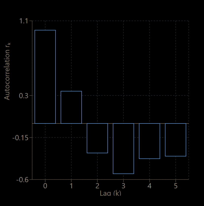
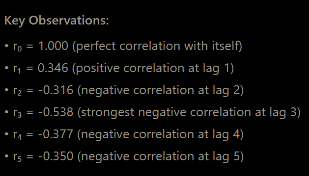
Strong negative correlation at lag 1 (ρ₁ = -0.877) indicates consecutive values tend to be opposite in nature
Moderate positive correlation at lag 2 (ρ₂ = 0.578) suggests some cyclical pattern
The process shows significant serial correlation, indicating the yields are not independent
Q3. Apply simple exponential smoothing with α = 0.5 to the series Y = [50, 52, 53, 54, 56]. The initial forecast is 50. Provide forecast for t = 6.
we are given:
series Y = [50, 52, 53, 54, 56]
alpha (α) = 0.5
initial forecast (F₁) = 50
we will apply simple exponential smoothing using the formula: Fₜ = α × Yₜ₋₁ + (1 − α) × Fₜ₋₁
goal: find forecast for t = 6 (i.e., forecast next value after 56)
F₄ = L₃ + T₃ = 116.6 + 8.24 = 124.84 final answer: forecast for t = 4 is 124.84
Q5. Given quarterly data Y = [30, 21, 29, 36, 42, 33, 41, 48], apply additive Holt-Winters method to compute L5, T5, S5 and forecast for t = 9. Use α = 0.5, β = 0.4, γ = 0.3, s = 4.
Holt-Winters Additive Method Solution
Given Data
Y = [30, 21, 29, 36, 42, 33, 41, 48] (8 quarters of data)
α = 0.5 (level smoothing parameter)
β = 0.4 (trend smoothing parameter)
γ = 0.3 (seasonal smoothing parameter)
s = 4 (seasonal period - quarterly data)
Find: L₅, T₅, S₅ and forecast for t = 9
Step 1: Initialize Parameters
Initial Level (L₁)
For additive model, we use the average of first season:
L₁ = (Y₁ + Y₂ + Y₃ + Y₄)/4 = (30 + 21 + 29 + 36)/4 = 116/4 = 29 Why: The initial level represents the deseasonalized average of the first complete seasonal cycle.
Q6. Apply Brown’s discounted regression (double exponential smoothing) with α = 0.5 to Y = [50, 52, 53, 54]. Compute level, trend, and forecast for t = 5.
Goal: Compute Level, Trend, and Forecast for t = 5
Step 1: What is Brown’s Double Exponential Smoothing?
This method is used when the time series has a trend, but no seasonality.
It smooths the data twice to estimate:
The Level (baseline value)
The Trend (upward/downward direction)
Then uses both to forecast future values
We use two smoothed series:
S₁(t) = single exponential smoothing
S₂(t) = double exponential smoothing
Step 2: Formulas Used
These are the core formulas:
4. S₁(t) = α × Yₜ + (1 − α) × S₁(t−1)
→ smooths the raw data once
5. S₂(t) = α × S₁(t) + (1 − α) × S₂(t−1)
→ smooths the smoothed data (S₁) again
6. Level (aₜ) = 2 × S₁(t) − S₂(t)
→ estimates current value based on double smoothing
7. Trend (bₜ) = (α / (1 − α)) × (S₁(t) − S₂(t))
→ measures the slope of the data (rate of change)
8. Forecast (Fₜ₊ₕ) = aₜ + bₜ × h
→ future forecast h steps ahead
Step 3: Initialization (Why?)
At t = 1, we need starting values.
We start by setting:
S₁(1) = Y₁ = 50
S₂(1) = Y₁ = 50
This is standard for Brown’s method (use first value as base).
Step 4: Apply the Smoothing Equations (Why?)
Now apply formulas from t = 2 to t = 4 to calculate S₁ and S₂.
At t = 2 (Y₂ = 52):
S₁(2) = 0.5 × 52 + 0.5 × 50 = 51 → Why? Smooth the actual value (52) with the previous smoothed value (50)
a₄ = 2 × S₁(4) − S₂(4) = 2 × 53 − 52.125 = 53.875 → Why? This estimates the base value by adjusting for double smoothing.
Trend (b₄):
b₄ = (α / (1 − α)) × (S₁(4) − S₂(4))
= (0.5 / 0.5) × (53 − 52.125) = 1 × 0.875 = 0.875 → Why? Measures how much the series is rising each step.
Step 6: Forecast for t = 5 (Why?)
We use: F₅ = a₄ + b₄ × 1 = 53.875 + 0.875 = 54.75 → Why? We're projecting one time step into the future using the current level + one unit of the trend.
Final Answer:
Level at t = 4 = 53.875
Trend at t = 4 = 0.875
Forecast for t = 5 = 54.75
Q7. Given AR(1) model Yt = 0.8Yt−1 + ϵt , with Y0 = 10 and ϵt = [0.5, −0.3, 1.0, −0.2, 0.1], compute Y1 to Y5.
AR(1) Model Step-by-Step Solution
Given Information
AR(1) Model: Yₜ = 0.8Yₜ₋₁ + εₜ
Initial Value: Y₀ = 10
Error Terms: εₜ = [0.5, -0.3, 1.0, -0.2, 0.1] for t = 1, 2, 3, 4, 5
Task: Compute Y₁ to Y₅
Understanding the AR(1) Model
What is AR(1)?
AR(1) stands for Autoregressive model of order 1, which means:
Auto: The variable depends on itself
Regressive: It's a regression on past values
Order 1: It depends on only 1 previous time period
Model Components Explained:
Yₜ: Current value we want to find
0.8: Autoregressive coefficient (φ₁) - shows how much current value depends on previous value
Yₜ₋₁: Previous period's value
εₜ: Random error/shock term for current period
Why This Formula Works:
The equation Yₜ = 0.8Yₜ₋₁ + εₜ tells us:
9. 80% of current value comes from the previous value (0.8Yₜ₋₁)
10. 20% is new information from the error term (εₜ)
11. Since 0.8 < 1, the series will gradually return to zero if no shocks occur
Step-by-Step Calculations
Step 1: Calculate Y₁
Given: Y₀ = 10, ε₁ = 0.5 Formula: Y₁ = 0.8Y₀ + ε₁ Calculation: Y₁ = 0.8 × 10 + 0.5 = 8.0 + 0.5 = 8.5 Why this step: We start with the initial condition Y₀ = 10 and apply the AR(1) formula to get the first forecasted value. The 0.8 coefficient means we take 80% of the previous value, then add the random shock.
Step 2: Calculate Y₂
Given: Y₁ = 8.5, ε₂ = -0.3 Formula: Y₂ = 0.8Y₁ + ε₂ Calculation: Y₂ = 0.8 × 8.5 + (-0.3) = 6.8 - 0.3 = 6.5 Why this step: Now Y₁ becomes our "previous value" and we apply the same logic. The negative error term (-0.3) pushes the value down from what it would have been with just the autoregressive component.
Step 3: Calculate Y₃
Given: Y₂ = 6.5, ε₃ = 1.0 Formula: Y₃ = 0.8Y₂ + ε₃ Calculation: Y₃ = 0.8 × 6.5 + 1.0 = 5.2 + 1.0 = 6.2 Why this step: The positive shock (1.0) is relatively large, boosting the value significantly above what the autoregressive component alone would give us (5.2).
Step 4: Calculate Y₄
Given: Y₃ = 6.2, ε₄ = -0.2 Formula: Y₄ = 0.8Y₃ + ε₄ Calculation: Y₄ = 0.8 × 6.2 + (-0.2) = 4.96 - 0.2 = 4.76 Why this step: The negative shock (-0.2) pulls the value down slightly from the autoregressive component (4.96).
Step 5: Calculate Y₅
Given: Y₄ = 4.76, ε₅ = 0.1 Formula: Y₅ = 0.8Y₄ + ε₅ Calculation: Y₅ = 0.8 × 4.76 + 0.1 = 3.808 + 0.1 = 3.908 Why this step: The small positive shock (0.1) slightly increases the value from the autoregressive component.
Summary of Results
Time (t)
Previous Value (Yₑ₋₁)
Error (εₜ)
AR Component (0.8Yₜ₋₁)
Final Value (Yₜ)
1
10.000
0.5
8.000
8.500
2
8.500
-0.3
6.800
6.500
3
6.500
1.0
5.200
6.200
4
6.200
-0.2
4.960
4.760
5
4.760
0.1
3.808
3.908
Key Observations
Pattern Analysis:
Mean Reversion: Without error terms, the series would decay toward 0 (since 0.8 < 1)
Shock Impact: Error terms create deviations from the smooth decay pattern
Persistence: Each value still carries 80% of the previous period's influence
Why AR(1) is Useful:
Economic Modeling: Many economic variables (GDP, inflation) show persistence
Financial Analysis: Stock prices, interest rates often follow AR patterns
Forecasting: Provides a simple way to model time-dependent data
Stationarity: When |φ₁| < 1 (like our 0.8), the series is stationary